A Step-by-Step Walkthrough Neural Networks for Time-series Forecasting

So you want to forecast your sales? Or maybe you would like to know the future price of bitcoin?

In both cases, you are trying to solve a problem known as “time-series forecasting”. A time-series is a sorted set of values that varies depending on time.

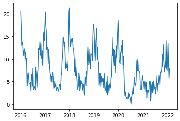
Example of a time-series. (Image by author)

No one can predict the future, but one can search in the past looking for patterns, and hope that those are going to repeat.

Guess what is very good in finding patterns? Neural networks (NNs from now on).

But which type of NN? I am going to test different kind of models on some artificially generated time-series. Each time-series will present a different combination of patterns, so that I can compare the different NN results.

After reading, you will know:

• how to choose a NN for time-series forecasting;
• how many past samples are needed to discover a pattern;
• which is the impact of noise on the prediction quality;

It is easy to say “Neural Networks”

There exist different kind of NN that can be applied to this use case.

• Multi-Layer Perceptron (MLP): the most common and simple. More about it here.
• Recurrent Neural Network (RNN): in literature, the most suited to time-series forecasting. They combine the information of the current observation, with the information of the previous observations. More about it here.
• Convolutional Neural Network (CNN): usually applied for Computer Vision, they are raising also for time-series forecasting. More about it here

It is not the purpose of this article going deep about each kind of network. Anyway, useful links are left for the reader that want to.

There are also different kinds of time-series, classifiable by the patterns that they present. It may happen that NNs perform differently depending on the time-series features.

Patterns and composition of time-series

Time-series presents mainly two types of patterns.

• Seasonality: the values periodically repeat.
• Trend: the values continue to increase or decrease.

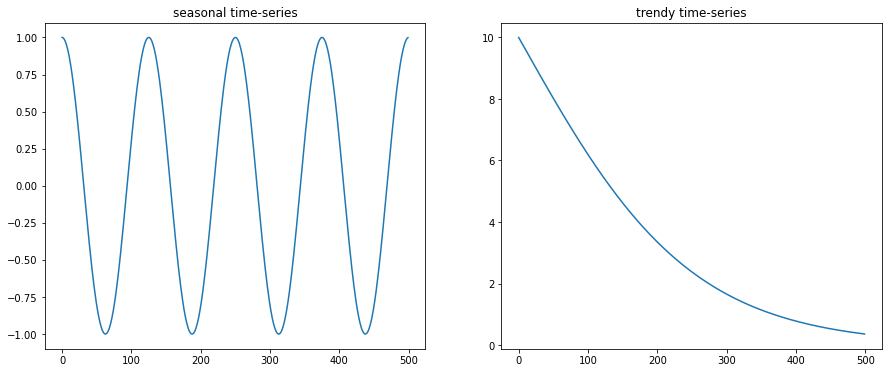
Examples of a seasonal and a trendy time-series. (Image by author)

A time-series forms from a non-linear combination of one or more trends, one ore more seasonalities and some noise.

1
2
3
y = f1(x) * trend1(x) + ... + fN(x) * trendN(x) +
    g1(x) * season1(x) ... + gN(x) * seasonN(x) +
    noise(x)

Trends and seasonalities are auto-correlated: future values depend on past values. The noise component may be instead totally random, or it could present a correlation with some feature external to the time-series.

I will conduct this analysis to test which NN is the best in finding seasonalities, trends and non-linearities.

During the experiment, the noise will be generated randomly. This means that there is nothing to discover that could predict the noise. It goes that our best models will present an average error very close to the amount of noise.

This is ok because I want to test how good is a model in discovering the patterns hidden by the noise.

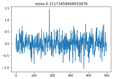
Examples of noise. (Image by author)

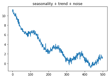
Examples of seasonality + trend + noise. (Image by author)

Neural networks benefits over statistical techniques.

Time-series forecasting is traditionally approached with statistical techniques, like ARMA (Auto-Regressive Moving Average), ARIMA (Auto-Regressive Integrated Moving Average), SARIMA (Seasonal Auto-Regressive Integrated Moving Average) or Facebook Prophet models. These require that you have some a-priori knowledge about the series.

• Is it the series stationary or not? (More about stationarity here)
• How many different seasonalities are present in the series (SARIMA).
• The differentiation order value to make the series stationary (ARIMA).
• Other…

Also, if you plan to predict only one next value, given a set of past values (many-to-one prediction), then the statical models need to be retrained every time a new value is added to the series.

In contrast, NNs don’t need to be retrained so frequently and don’t require any a-priori knowledge. In addition, it is quite straightforward to add external information that may correlate to the noise generation (multi-variate input).

Experiments

You can find the entire notebook here

You can also download and alternative version from here. Install this requirements.txt if you want to run it locally.

Let’s start by defining a function to generate a wave, and use it to plot a wave of period 10 with 520 samples and amplitude 1.

I will start from the most simple MLP with one hidden layer of 5 neurons, an output layer of 1 neuron, and an input layer of the same size as the input. Which input?

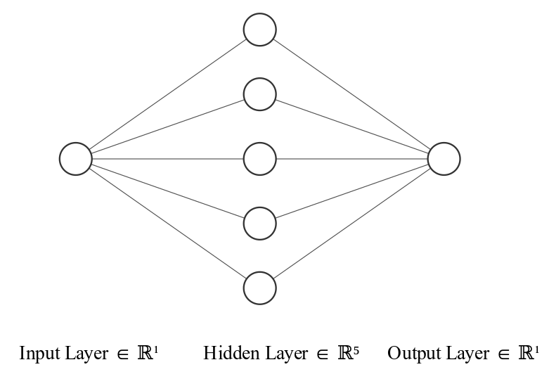
The simple MLP. (Image generated with NN-SVG)

I want to forecast the value of the series at time t, let’s call it y(t). Then I will input to the NN the values y(t-N)...y(t-1) for N <= t and N > 1. I will call this input “lags”. I want to see how the network performs, feeding it with only the first lag y(t-1).

Data preparation

NNs better perform with dataset values ranging between [0, 1] (as explained here). Then let’s apply a scaling function.

After, let’s define a function to prepare our dataset. It will output a pandas DataFrame where each row is an input sample, and the columns are the lags together with the actual output value.

The last operation is to split the dataset into train and test sets. I will use the first 60% of the dataset to train, and the left 40% to test.

Model Hyper-parameters and evaluation environment

I will use Keras backed by Tensorflow.

Let’s consider some of the hyper-parameters that I adopt for training. I will use Adam as the gradient descent optimizer and mean squared error for measuring the training error. The batch size will be the default value of 32 (empirically choosen). The model will train for a maximum of 200 epochs, early stopped if no further improvement is observed for 30 consecutive epochs.

I choose the Elu activation function because it makes the models training more stable. I experienced the improved stability during tests, not reported here for brevity. For the convolutional layer I use instead the Relu activation function, because I empirically observed better performance. The output has a linear activation function.

The prediction is going to be compared with the actual test values, measuring the error with the root mean squared error.

I will also compare the NN prediction, with two naive predictors. The average value of the test set (not usable as a predictor, as it uses future values) and the test set shifted by 1 time lag (i.e. y'(t+1) = y(t)).

There is always a certain level of randomness when training a model. This makes it very difficult to understand the effects of changing the hyper-parameters.

One countermeasure is to train the same model many times and then average the results. In this experiment, I will train the models 5 times.

The quality of the model is given by it’s average RMSE and the Standard Deviation (std) of the errors. A high quantity of std means that the model is not stable in its training. (i.e. Different trainings may result in models that performs very differently.)

Model training (finally 😅)

Let’s train our simple MLP

The result is not satisfying. The predictions are just the test series shifted by one lag.

I can think of changing 3 things to improve the prediction:

• the number of hidden neurons;
• the number of training epochs;
• the number of lags.

Let’s reason for a while.

It is straightforward to exclude the number of epochs, looking at the above graphics of the training losses. All of the 5 trainings stopped early, after a consistent number of epochs with an error close to 0 and no improvements.

Now zoom-in our sinusoid, near one of the higher peaks.

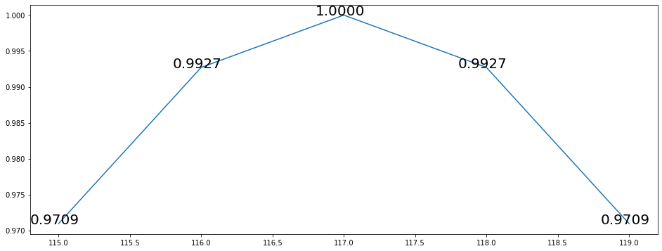
Zoom-in of the sampled sin function near to 1. (Image by author)

You can notice that the same values repeat both ascending and descending. The same input y(t) can output two different y(t+1) values. It doesn’t exist a unique relation between inputs and outputs.

We can conclude that we need at least two input lags to learn the function.

We observed that a simple MLP with one hidden layer, can learn a sinusoidal function, with a minimum input of 2 lags.

Let’s do some noise!

What happens if I introduce noise?

We should not be surprised to see that the prediction looks again laggy. Indeed, the RMSE is even worst than the shifted baseline. Given a noise with an std value 0.1, we should expect an RMSE value as close as possible to 0.1.

How many lags do we need to discover the pattern hidden by the noise?

Let’s try to see what happens with 4 lags.

Better, but no pattern looks to have been discovered. Let’s now try again with 10 and 20 lags.

With 10 lags the prediction gets better but it is still a bit noisy.

With 20 lags it finally looks like the model found our pattern again. Also the average is very close to the target value of 0.1.

You promised MOAR networks!!

Yes, I did. So, let’s define a helper function to test many different models together. Namely:

1. Our simple MLP
2. A deeper MLP with 3 hidden layers
3. The same as 2, but with a Dropout layer, to see if it helps
4. Some Recurrent NN:
   • A Simple RNN
   • A model with 2 stacked RNN layers
   • A Long-Short Term Memory (LSTM). A special kind of RNN that can keep information more distant in the past.
   • A Gated Recurrent Unit (GRU). Has similar properties of an LSTM, but requires less computation effort.
5. A Convolutional NN
6. The same as 5 but with a Dropout layer.

And here are the results.

Looks like complicating the model doesn’t actually improve.

Will it be the same also with more complicated patterns?

Experiments with different time-series.

I am going to observe the NN behavior, against series that present the following features:

• Fading Wave: a wave that changes its amplitude as time passes. With some noise.
• Complex series: a series that is composed of 3 waves with different frequencies and amplitude, one trend, and a significative amount of noise.
• Realistic series: a series that is composed of many waves, one trend, and a very high amount of noise. I call it “realistic” because it is built looking at the spectrum of its Fourier Transform. The purpose is that it presents many components, with no one clearly prevailing over the others (similar peaks).
  This should mimic the FT Spectrum of a real time-series of the sales of a product.

Fading Wave: Noise 0.1. RMSE 0.1914 for the mean. RMSE 0.125 for the shift:

Complex Series: Noise 3. RMSE 4.008 for the mean. RMSE 4.196 for the shift:

Realistic series: Noise 6. RMSE 8.14 for the mean. RMSE 11.04 for the shift:

Fading Wave results: Noise 0.1. RMSE 0.1914 for the mean. RMSE 0.125 for the shift

Complex series results: Noise 3. RMSE 4.008 for the mean. RMSE 4.196 for the shift

Realistic series results: Noise 6. RMSE 8.14 for the mean. RMSE 11.04 for the shift

The models do very well with the “Fading series”. Even less than the target value 0.1. We can deduce that all the models can discover that the pattern changes in time.

Looks like in presence of more complex patterns, CNN does the best job. While the RNN flavors are not performing better than the others. This is not what we would expect from the literature.

“Realistic series” presents a very large amount of noise, and all the networks have an average error higher than 7, which is quite far from the target value of 6. This suggests that in a real environment we should try to add more information external to the time-series, to search for patterns that correlate to the noise. For example, if we are analyzing sales of a product that has a categorical classification, adding the sales of other products of the same category may help.

It is surprising that even the simple and the deep MLPs always return quite good results.

The dropout level in the CNN helps in lowering the Standard Deviation.

More information from the past

Is there any information coming from the series itself that we are not yet considering?

Let’s have a look at the auto-correlation plots:

We are currently considering 20 lags, but there is some correlations with the lags older the 20. Instead of highering the number of lags, we could try to add past values in an aggregated form. Let’s add the average values of the 4 previous lags, and of the 12 previous lags.

In the “Complex series” there is a seasonality that repeats about every 25 lags. Let’s try to catch these kinds of seasonalities by adding the averaged values (1 lag, 4 lags, and 12 lags), shifted by the number of lags that corresponds to the higher auto-correlation (after the 12th lag).

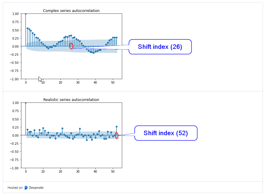
Shift indexes. (Image by author)

We now adapt the CNN to be 2D CNN instead of 1D, as now we are passing 20 lags for each sample, with 6 features vector each. We also add one more model: a CNN with 2 Convolutional layers, separated by one pooling layer.

Let’s have a look at the results:

Complex series results: Noise 3. RMSE 4.008 for the mean. RMSE 4.196 for the shift

Realistic series results: Noise 6. RMSE 8.14 for the mean. RMSE 11.04 for the shift

All the models improve. In the “Realistic series” the RNN model improve a lot with LSTM becoming the best performer. The noise value is now closer to the target noise value 6. Also in the “Complex series” the LSTM gives a result comparable to the CNN, but more stable.

The Deep CNN model does not give any significant improvement.

Conclusion

During this analysis, I demonstrate that a simple MLP can learn a sinusoid, with an input of 2 lags.

When noise is introduced, we need 20 lags to learn the underlying pattern. We then observed that more complicated NN (RNN and CNN) does not improve the results for a sinusoid with noise.

We then observed that all the models can discover even more complex patterns. CNN does the best with complex patterns, and a Dropout level helps improve the result and the model stability.

CNNs start having some difficulties when the series presents too many patterns and a high amount of noise.
I demonstrated that feeding the NN with aggregated information from the past improves a lot the results. Finally, LSTM become one of the best performers, as we would have expected.

If we would have to choose a model for a real-world time-series, a good idea would be to choose an ensemble of CNN with a Dropout layer and an LSTM. The model should be input with at least 20 lags and some averaged values from the past.

Another good idea would be to add more information external to the time-series values. The attempt is to find any measurable correlation with the noise.